Project 3: Classification
Introduction
Nobody likes spam in their inbox. While it seems that we have this problem mostly figured out, the occasional junk message still slips through the cracks. The goal of this project is to think about this problem in multiple ways and ground the general principles of classification and supervised learning.
The dataset we will be using comes from the Enron corpus, a large bank of emails labeled ham (valid) or spam (junk). We will provide you with a large subset of the entire dataset in order to develop and test your classifiers, but we will also run your code on held-out data to ensure that your solutions generalize.
The dataset we will be using comes from the Enron corpus, a large bank of emails labeled ham (valid) or spam (junk). We will provide you with a large subset of the entire dataset in order to develop and test your classifiers, but we will also run your code on held-out data to ensure that your solutions generalize.
Files & Setup
Setup
Run cs141_install classification to retrieve the stencil code and data for this project. Note: This project makes use of the Python libraries Numpy, Matplotlib, and Scikit-learn. If you are not working on department machines, you may need to install these to complete the project.
Files
There are a number of python files provided for you. They are detailed below.
Within the data folder, we also have a number of files.
| features.py | Contains code for loading in the data from file. |
| classifiers.py | The stencil code for the classifiers you will be writing. There is one currently implemented. See the Simple Classifier section below for details |
| classify.py | This is the file you will run to run the classifiers. More details follow. |
Within the data folder, we also have a number of files.
| train.txt | This file contains a bank of emails that will be used to train the models. |
| test.txt | This file contains a bank of emails that will be used to evaluate the accuracy of the models. |
| train_small.txt | A subset of train.txt that allows for much faster development. The ratio of ham emails to spam emails is roughly consistent with the full set. |
| test_small.txt | A subset of test.txt. |
Loading Data and Testing
Loading Features - The constructor of the EmailFeatures class in features.py (let's call the instance feats) takes in an optional file location argument and builds an object with three main fields. feats.X is a list of lists, where each element in the higher-level list represents the words of a given email in list form. feats.y is a list whose elements are the strings "ham" and "spam", the class that corresponds to the same-indexed email in feats.X. Additionally, feats.vocabulary contains a set of all the words that were encountered in the dataset.
Running & Testing the Classifiers - The bayesian classifiers (NBSpamClassifier and BigramClassifier) take in an entire EmailFeatures object, which should then be used to train the model (more details follow in the implementation section). For testing both the models that learn (the bayesian ones) and those that do not, one email is passed at a time into the classify method of the model. This is handled by the validate method in the classifiers.py file.
The the python script classify.py runs the project. It takes two arguments. The first is a mandatory argument to specify which portion of the project should be run. The second is an optional argument that specifies if you would like to run the project using the trimmed-down datasets for faster development. Run python classify.py to see all the options.
The the python script classify.py runs the project. It takes two arguments. The first is a mandatory argument to specify which portion of the project should be run. The second is an optional argument that specifies if you would like to run the project using the trimmed-down datasets for faster development. Run python classify.py to see all the options.
Implementation
Simple Classifier
Before we dive into sophisticated methods that learn from data, we are going to use a simple decision rule to get acquainted with the problem. The goal is simply to assign a label to each email, and there are many ways you could make that decision. One possibility would be to mark all of them as ham, though we intuit that that is not a very good decision rule. Marking every third email spam would probably give slightly better results, but it is not much more satisfying than the first rule. We want to encode some "smarts" (this is a course in Artificial Intelligence after all) in making the ham/spam decision.
The classifier defined by the SimpleSpamClassifier class uses a simple rule to make decisions. It is modeled by the following decision tree.

Your goal is to write a classifier that performs better than SimpleSpamClassifier in the
BetterSpamClassifier class. Feel free to get creative, but any improvement over the performance of SimpleSpamClassifier will be awarded full credit. Please give an explanation of your classifier in your readme.
To run the simple classifier, use python classify.py simple.
To run your better classifier, run python classify.py better. This will case a NotImplementedError until you fill in the BetterSpamClassifier in classifiers.py.
See the grading section for expected accuracy values for these and the other classifiers.BetterSpamClassifier class. Feel free to get creative, but any improvement over the performance of SimpleSpamClassifier will be awarded full credit. Please give an explanation of your classifier in your readme.
To run the simple classifier, use python classify.py simple.
To run your better classifier, run python classify.py better. This will case a NotImplementedError until you fill in the BetterSpamClassifier in classifiers.py.
Naive Bayes Classifier
While the SimpleSpamClassifier encodes some human intelligence, it could be easily thwarted. Thus, we are going to implement a more sophisticated method that learns from the training data. The general form of this problem is supervised learning, or learning a function from labeled training data. At test time, we will use this function along with a basic decision rule to classify the test dataset. We will further investigate the decision rules in the last section of this project.
The model we will be using is a naive bayes model, which is one of the more simple and intuitive supervised learning models. In naive bayes, we make an assumption that allows us to simplify the model considerably. The features (the representation of the data on which you are learning the model) are considered to be conditionally independent. There are infinitely many feature representations we could use. For instance, we could use the length of the email or the sender as potential features.
However, for this portion of the assignment, we are going to use a "bag of words" model. That is, we treat each email as an unordered list of words and use these words as features for our classifier.
Mirroring the variables from the EmailFeatures class, we define:
- X - the set of test features (emails)
- thus, a vector x (one element of X) represents the words in an email
- y - the vector labels associated with the email
- thus an individual y is a label associated with one x
Recall bayes theorem:
 |
| Equation 1 |
- p(y|x) is the posterior. We would like to compute this for each class.
- p(x|y) is the likelihood. That is, given the class, what is the likelihood of seeing the data?
- p(y) is the class prior, some encoding of how likely each class is not considering the data at hand.
- p(x) is the marginal. In other words, this is the probability of seeing the data over all the possible choices for y. Since this is equivalent in all of the classes, we do not compute it, and instead use
 |
| Equation 2 |
to make our decisions. This leaves the question of how we compute p(x|y) and p(y). Recall that this model assumes conditional independence of the features. If we define n to be the number of features in x, we can rewrite this formula as:
 |
| Equation 3 |
where we will use the following estimators for p(y) and p(xi|y):
Assuming that the main goal is accuracy, the proper decision rule is then to choose the class that yields a higher value for the posterior, p(y|x).
Your task in building this classifier (NBSpamClassifier) is twofold. First you must train the model to learn the values for Equations 4 and 5. This should be done when the model is constructed. Then, you must use those values to compute the posterior for each class and return "ham" or "spam" as the chosen categorization for each test email. See the stencil code for details.
There are three caveats when it comes to computing the posterior.
To run this portion of the assignment, use python classify.py naive
 |
| Equation 4 |
 |
| Equation 5 |
Your task in building this classifier (NBSpamClassifier) is twofold. First you must train the model to learn the values for Equations 4 and 5. This should be done when the model is constructed. Then, you must use those values to compute the posterior for each class and return "ham" or "spam" as the chosen categorization for each test email. See the stencil code for details.
There are three caveats when it comes to computing the posterior.
- Numerical underflow - many of the p(xi|y) values are very small, and depending on the length of an email, the posterior can become too small to be represented by python floats. There is, however, a simple solution to this issue: taking the log of the entire Equation 3.
Thus, instead of computing Equation 3, you want to instead compute:
Equation 6
While this changes the numbers themselves, taking a log is a monotonic transformation, so which class's posterior value is greater will be preserved. - Words that do not appear in training - If a word does not appear in the training dataset, it cannot provide any useful information at test time. Additionally, trying to log the likelihood estimator of that word (which should be 0) will lead to numerical errors. To correct for this, before adding a word's logged likelihood, be sure to check that it occurred in the training dataset (the EmailFeatures.vocabulary field provides an easy way to check this).
- Words that appear in only one training class - There will be some words that occur in only one of the training classes. If a word appears in only one class, it is probably a good representative feature of that class. Therefore, to ignore the word entirely would not be a good solution. On the other extreme, you could immediately declare the email of the representative class, but that would not suffice if the email had one of such type of word from each class.
The approach that we want you to use (which comes from computational linguistics) is called smoothing. This approach accounts for the possibility of not seeing a feature in the training examples of a class by substituting a value for the 0 logged likelihood. There are many smoothing methods, which apply to different problem domains.
Since we expect these events to happen infrequently in the case of email, we will use a simple approach. Define a class-independent value (we'll call this epsilon). A good epsilon value is:
Thus, this value would be smaller than seeing a word only once in wither class. Substitute this epsilon value instead of computing Equation 4 for that word.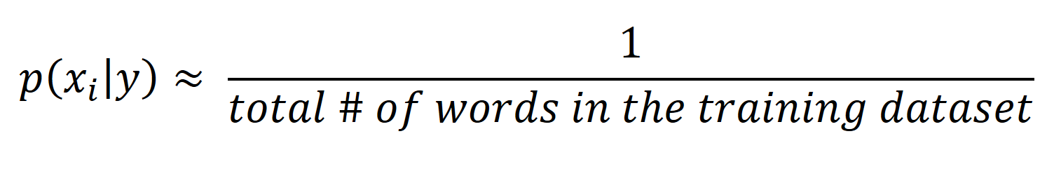
Equation 7
To run this portion of the assignment, use python classify.py naive
Playing with Features
As is mentioned above, there are many possible selections for the features used in the model. The previous section considered only single words as features. In computational linguistics, these features are known as "unigrams". In this section of the project, we will also consder "bigrams". or two-word features. For example in the sentence "My name is Wall-E.", the unigrams are {"My", "name", "is", "Wall-E"}, while the bigrams are {(My,name), (name,is), (is,Wall-E)}. Using bigrams allows us to encode more meaning about the words in relation to the other words, which makes our classifier even more accurate.
In this portion of the assignment, we would like you to make another naive bayes classifier, which uses both unigrams and bigrams as features. Be sure to account for the caveats from the previous section as they apply to bigrams as well as unigrams.
To run this portion of the assignment, use python classify.py bigram
Thresholding & ROC Curves
The final part of this project will look into decision rules. There are two extremes for decision rules: marking all emails as ham and all as spam. We also have a nuumber of possibile choices between these two rules. The rule we used above was to choose the class that produced a higher posterior probability. This rule maximizes accuracy, which is in general a good metric. However, depending on your problem domain, it may be better to consider altering the threshold by which you make decisions. For example, if a classifier is some sort of determinant of disease, it may be better to err on the side of over-diagnosing to ensure that all potentially-affected patients receive further inspection by a doctor.
The spectrum of decision rules can be visualized by using an Receiver Opertating Characteristic (ROC) Curve. The ROC Curve compares the tradeoffs in changing thresholds for a binary classifier. We have been referring to the classes as "ham" and "spam", but to speak generally and match the terminology, assume one class is "positive" and the other "negative". Let us define a few metrics:
- True Positive (TP) - A test example is positive and is classified as such
- False Positive (FP) - A test example is negative and is classified as positive
- True Negative (TN) - A test example is negative and is classified as such
- False Negative (FN) - A test example is positive and is classified as negative
- True Positive Rate (TPR), or sensitivity - TP/(TP + FN)
- False Positive Rate (FPR), or fall-out - FP/(FP + TN)

The dotted line represents what you could expect from a completely naive classifier, one that arbitrarily assigned confidence values. Classifiers are often judged but the area under the curve (AUC), which is 0.5 for the dotted line. The AUC of a good classifier is always above 0.5 (otherwise the classifier should reverse the labels it is applying). The ideal classifier would have an AUC of 1, meaning that there is some decision rule for which its TPR is 1 (all positive examples correctly classified) and its FPR is 0 (no negative examples misclassified as positive).
Your final task is to make a ROC curve for your NBSpamClassifier. We have provided stencil code for this portion of the assignment in the plot_roc method of classify.py. This relies on the ROC module from scikit-learn, a python machine learning library. The usage is explained in the stencil code, and there is an example on the scikit-learn website. Namely, you need to provide to the roc_curve method 2 or 3 arguments:
- The test label. These need to be converted from "spam" and "ham" to 0 and 1. Which maps to which is going to depend on which class your confidence values (see below) are indicating. The provided convertmethod will do this for you, and takes an optional second argument of the positive label (if you don't want it to be "spam").
- A list of confidence values or probabilities. Since the probabilities are logged, the easiest way to do this is to subtract the "negative" logged posterior from the positive one. Which class is positive/negative is determined by:
You may need to write another method in NBSpamClassifier to provide the cofidence values. As was mentioned above, the AUC should be greater than 0.5. If this is not the case, try flipping the third argument.
To run this portion of the assignment, use python classify.py roc
Consider two users, C3PO and R2D2. C3PO is easily bothered by spam, so given the choice, he would prefer to miss a few messages rather than have spam in his inbox. On the other hand, R2D2 can tolerate a bit of spam but does not want to miss a single ham email. A classifier that can achieve the top-left point of the Which side (bottom-left or top-right) does each of C3PO and R2D2 prefer? Explain in a sentence or two. Please include your answer to this question in your readme.
<Accuracy Expectations>
Grading
The project will be evaluated as follows:
- Simple Classifier (w/explanation): 7 points
- Unigram Naive Bayes Classifier: 30 points
- Bigram Naive Bayes Classifier: 10 points
- ROC curve (w/ explanation): 13 points
Expected Accuracy Table (all approximate):
| Small Datasets | Full Datasets | |
| Simple | 58% | 76% |
| Better | -- | >76% |
| Unigram Naive Bayes | 91% | 88% |
| Bigram Naive Bayes | 92% | 94% |
No comments:
Post a Comment